I recently needed to plot some polar data for a project at work, and the data happened to be 3-dimensional. In addition to the standard rotation and radius, it had a third dimension that corresponded to a strength metric. Unfortunately, Mathematica (my tool of choice for data manipulation and plotting) lacks native support for 3D plotting in the polar coordinate system. It does, however, have excellent support for list/matrix manipulation, so I was able to put together this one-liner to produce a 3D plot from a N x 3 matrix of θ, r, h coordinates:

ListPolarPlot3D[data_, opts___] := Module[{polarConvert}, polarConvert[coords_] := {coords[[2]]*Cos[coords[[1]] Degree], coords[[2]]*Sin[coords[[1]] Degree], coords[[3]]}; ListPlot3D[Map[polarConvert, data], Evaluate[opts]]]

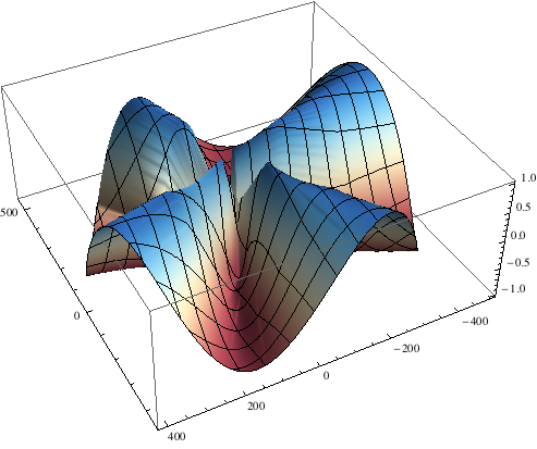
After pasting that into your Mathematica notebook, you can easily generate 3D plots of polar coordinate data by calling ListPolarPlot3D. For example:

ListPolarPlot3D[Table[{n, n/2, Sin[n*4 Degree]}, {n, 0, 1080}],  ColorFunction -> "RedBlueTones"]

Gives you this:

Example Polar Plot

Breakdown

Here’s what each part of the snippet does:

ListPolarPlot3D[data_, opts___] :=  Define a function called `ListPolarPlot3D` that takes a variable number of arguments. Store the first argument in the `data` variable, and all the others in the `opts` variable. The triple-underscore means "zero or more arguments".

Module[{polarConvert},  Create a local scope for the `polarConvert` function so that it doesn't interfere with anything in the global scope that might be called `polarConvert`.

polarConvert[coords_] := {coords[[2]]*Cos[coords[[1]] Degree], coords[[2]]*Sin[coords[[1]] Degree], coords[[3]]}; Use the identities `x = r × cos(θ)` and `y = r × sin(θ)` to convert the polar coordinates to Cartesian, and leave the `y` coordinate alone

ListPlot3D[Map[polarConvert, data], Evaluate[opts]]] This does three things. `Map[polarConvert, data]` applies the polar coordinate conversion function to each coordinate in the data, then returns the converted dataset. `Evaluate[opts]` allows us to pass in a List of options to `ListPlot3D` bypassing the `HoldAll` attribute that `ListPlot3D` has by default. `ListPlot3D` takes the converted cartesian data and evaluated options and generates a 3D plot from them. The final closing bracket closes the `Module` and returns the `ListPlot3D`.

Modifications

It’s pretty easy to tweak the snippet to suit your needs. Here are a couple of examples:

Use radians instead of degrees

ListPolarPlot3D[data_, opts___] := Module[{polarConvert}, polarConvert[coords_] := {coords[[2]]*Cos[coords[[1]]], coords[[2]]*Sin[coords[[1]]], coords[[3]]}; ListPlot3D[Map[polarConvert, data], Evaluate[opts]]]

Render the data as points rather than a surface

ListPolarPointPlot3D[data_, opts___] := Module[{polarConvert}, polarConvert[coords_] := {coords[[2]]*Cos[coords[[1]] Degree], coords[[2]]*Sin[coords[[1]] Degree], coords[[3]]}; ListPointPlot3D[Map[polarConvert, data], Evaluate[opts]]]

Limitations

There are a few things to note when using this technique. First, Mathematica wants to automatically scale the axes by default. This can result in improperly displayed graphs if the scale for the x and y axes is different. I recommend setting your xy scale explicitly (i.e. PlotRange -> {{-10, 10}, {-10, 10}, Automatic})).

Second, you’re going to have Cartesian axes displayed. Short of really digging into Mathematica’s Graphics3D implementation, there’s really no good way around this as the way that the whole technique works is by mapping the polar data into the Cartesian plane.